SAP Data Warehouse

A.                Data Warehousing Concept.

Data warehousing forms the basis of an extensive business intelligence solution that allows converting data into valuable information. Integrated and company-specific data warehousing provides decision makers in your company with information and knowledge about goal-oriented measures that will lead to the success of the company. For data from any source (SAP or non-SAP sources) and of any age (historic or current), data warehousing in BI allows: Integration (data acquisition from source system), Transformations, Consolidations, Clean up, Storage, Retrieval for analysis and interpretation.

The architecture of data warehouse differentiates between the following layers:

• Persistent staging area (PSA): After it is extracted from source systems, data is transferred to the entry layer of the data warehouse, the persistent staging area (PSA).
• Data Warehouse: The result of the first transformations and clean up is saved in the next layer, the data warehouse.
• Architected data marts: The data warehouse layer provides the most multidimensional reporting structures. These are also called architected data marts.
• Operational data store: As well as strategic reporting, a data warehouse also supports operative reporting by means of the operational data store.

Pic. 1 : Architecture of Data Warehouse

An enterprise data warehouse (EDW) is a company-wide data warehouse that is built to include all the different layers. An organizational-wide, single and central data warehouse layer is also reffered to as an EDW. An EDW has provide flexible structures and layers so that it can react quickly to new business challenges (such as changed objectives, mergers, acquisitions).

The structure and running of a data warehouse in general, and an enterprise data warehouse in particular, are highly complex and cannot be tackled without the support of adequate tools. Data warehousing as an element of Business Intelligence in SAP NetWeaver provides: Data staging, modeling layer architecture, transformation, modeling the data flow, and staging data for analysis.

B.                 Data Store Object (DSO).

The DataStore object with SAP NetWeaver 2004s BI is the successor object of the former ODS-Object. The major enhancement is that there are various types to define the DataStore Object: standard datastore object, datastore object for direct update, and write optimized datastore object. Below show the differences between the datastore object types:

1. 1.      Standard DataStore Object.

The standard DataStore object is filled with data during the extraction and load process in the BI system. A standard DataStore object is represented on the database by three transparent tables:

• Activation Queue: Serves to save DataStore object data records that are to be updated, but that have not yet been activated. The data is deleted after the records have been activated. The following key fields are defined technically: Request surrogate ID, Packaged ID, and record number.
• Active Table: A table containing the active data (A table).
• Change Log: Contains the change history for the delta update from the DataStore object into other data targets, such as DataStore objects or InfoCubes.

1. 2.      DataStore Object for Direct Update.

A datastore object for direct update contains the data in a single version. Data is stored in precisely the same form in which it was written to the DataStore object for direct update by the application. In the BI system, you can use a DataStore object for direct update as a data target for an analysis process. The DataStore object for direct update is also required by diverse applications, such as SAP Strategic Enterprise Management (SEM) for example, as well as other external applications. DataStore objects for direct update ensure that the data is available quickly. The data from this kind of DataStore object is accessed transactionally, that is, data is written to the DataStore object (possibly by several users at the same time) and reread as soon as possible.

1. 3.      Write-Optimized DataStore Object.

Write-Optimized DataStore Object is DataStore object that only consists of one table of active data. Data is loaded using the data transfer process. Data that is loaded into write-optimized DataStore objects is available immediately for further processing.

You use write-optimized DataStore objects in the following scenarios:

• You use a write-optimized DataStore object as a temporary storage area for large sets of data if you are executing complex transformations for this data before it is written to the DataStore object. Subsequently, the data can be updated to further (smaller) InfoProviders. You only have to create the complex transformations once for all data.
• You use write-optimized DataStore objects as the EDW layer for saving data. Business rules are only applied when the data is updated to additional InfoProviders.

The system does not generate SIDs for write-optimized DataStore objects and you do not need to activate them. This means that you can save and further process data quickly. Reporting on the basis of these DataStore objects is possible. However, we recommend that you use them as a consolidation layer, and update the data to additional InfoProviders, standard DataStore objects, or InfoCubes.

C.                InfoSet.

InfoSet describes data sources that are defined as a rule as joins of DataStore Objects, standard InfoCubes and/or InfoObject (characteristic with master data). A time-dependent join or temporal join is a join that contains an InfoObject that is a time-dependent characteristic. An InfoSet is a semantic layer over the data sources. Unlike the classic InfoSet, an InfoSet is a BI-specific view of data.

Some more new functionality enhances the objects : InfoCubes are possible for join, time dependencies can be define for Data Store Object and InfoCubes to treat these object in a way as time dependent attributes, and some additional function are enhanced within the InfoSet Builder (RSISET).

• InfoSet Concept – Join.

A join condition determines the combination of individual object records that are included in the results set. Before an InfoSet can be activated, the join conditions have to be defined in such a way (as equal join condition) that all the available objects are connected to one another either directly or indirectly. In InfoSet concept have two join conditions. There are Inner join and Left Outer Join.

• Time Dependencies In InfoSet – Temporal Join.

Temporal join used to map a period of time. Temporal join combines InfoCubes data with time-dependent master data and joins the time dimension to the validity reports.

Temporal operands are time characteristics, or characteristics with a date, that have an interval or key date defined for them. They influence the results set in the temporal join.

• Key Date.

Depending on the type of characteristic, there are various ways to define a key date:

~        Use first day as a key date.

~        Use last day as a key date.

~        Use a fixed day as a key date (a particular day from the specified period of time).

~        Key date derivation type: you can specify a key date derivation type that you defined using EnvironmentàKey Date Derivation Type.

 

• Time Interval.

You can set time intervals for time characteristics that describe a period of time with a start and end date. Start and end dates are derived from the value of the time characteristic. In the context menu of the table display of the InfoProvider, choose Define Time-dependency. The system adds extra attributes (additional fields) to the relevant InfoProvider. These have the start and end dates from (0DATEFROM) and to (0DATETO).

D.                Remodeling Toolbox.

Remodeling used to change the structure of the object, without losing data. A remodeling rule is a collection of changes to your InfoCube. These changes are executed at the same time. For InfoCubes, you have the following remodeling options

• Characteristic Conversion.

~        Add/Replace characteristic initially filled with: constant (e.g. dummy characteristic value), Attribute of an InfoObject of the same dimension, the same value of another InfoObject of the same dimension, Customer exit (for customer-specific coding of the initial value).

~        Delete characteristic.

• Key Figure Conversion.

~        Add key figure initially filled with: constant (e.g. “0”), customer exit (for customer-specific coding of the initial value).

~        Replace key figure: customer exit (for customer-specific coding of the initial value).

~        Delete key figure.

The remodeling schedule has two types. There are schedule the remodeling rule or start it immediately, periodic scheduling not useful. The status of a request and the corresponding steps are displayed in the monitor. When a remodeling is executed, errors may occur for several reasons:

• Problems with database (insufficient table space, duplicate keys, partitioning, and so on).
• Problems with the application server caused by large volumes of data (timeout, and so on).
• Problems caused by conversion routines.

If an error occurs, you can restart a particular step or the whole request from the monitor. To do this, choose Reset Step in the context menu for a step, or Reset Request in the context menu for the request. Then choose Restart Request in the context menu for the request.

E.                 Business Content (Content Analyzer).

Check program are provided to customer to analyze inconsistencies end error of customer defined information model (InfoObject, InfoProvider, etc). With transaction code RSBICA you can:

• Schedule these delivered check programs for the local system or remote system via RFC connection.
• Customize the scheduling options.
• Display the result of check programs by several grouping possibilities, several filter options, priorities.

Check categories means different check programs. For details of what the check programs are doing please refer to the appendix.

 

A priority can be assigned to every check category. A default priority setting will be delivered by SAP. It can be overwritten by customers. 4 priority settings are possible:

• Very High (1).
• High (2).
• Medium (3).
• Low (4).

The monitor will give you an overview about the result:

• The priority fields provide an aggregated view to the objects listed and the result container.
• In the “last update” field, the date and time of the oldest objects which is available in the result container is displayed.
• The date and time of the objects will be set during the runtime of the check programs. The values in the monitor will change if the filter restrictions have been changed.

F.                 Concept for BI Data Sources.

Set of fields that provide the data for a business unit for data transfer into BI. From a technical viewpoint, the Data Source is a set of logically-related fields that are provided to transfer data into BI in a flat structure (the extraction structure), or in multiple flat structures (for hierarchies). There are four types of Data Sources:

• Data Sources for Transactional data.
• Data Sources for Master Data (Attributes).
• Data Sources for Master Data (Texts).
• Data Sources for Master Data (Hierarchies).

Data Sources supply the metadata description of source data. They are used for extracting data from a source system and for transferring data into BI. The following image illustrates the role of the Data Source in the BI data flow:

The data is loaded into BI from any source in the Data Source structure. An InfoPackage is used for this purpose. You determine the target into which data from the Data Source is to be updated during the transformation. You also assign Data Source fields to target object InfoObjects in BI.

Below explain the differences between Data Sources vs. 3.x Data Sources:

• 3.x Data Sources.

Data Sources were previously known as Data Source replicates (object type R3TR ISFS) in the BI system. The transfer of data from this type of Data Source (referred to as 3.x Data Sources below) is only possible if the 3.x Data Source is assigned to a 3.x Info Source and the fields of the 3.x Data Source are assigned to 3.x Info Source InfoObjects in transfer structure maintenance. A PSA table is generated when the 3.x transfer rules are activated, thus activating the 3.x transfer structure. Data can be loaded into this PSA table. If your dataflow is modeled using objects that are based on the old concept (3.x Info Source, 3.x transfer rules, 3.x update rules) and the process design is built on these objects, you can continue to work with 3.x Data Sources when transferring data into BI from a source system.

• Data Sources.

A new object concept is available for DataSources. It is used in conjunction with the changed objects concepts in data flow and process design (transformation, InfoPackage for loading to the PSA, data transfer process for data distribution within BI). The object type for a DataSource in the new concept – called DataSource in the following – is R3TR RSDS. In DataSource maintenance in BI, you specify which DataSource fields contain the decision-relevant information for a business process and should therefore be transferred. When you activate the DataSource, the system generates a PSA table in the entry layer of BI. You can then load data into the PSA. You use an InfoPackage to specify the selection parameters for loading data into the PSA. In the transformation, you determine how the fields assigned to the BI InfoObjects. Data transfer processes facilitate the further distribution of data from the PSA to other targets. The rules that you set in the transformation are applied here.

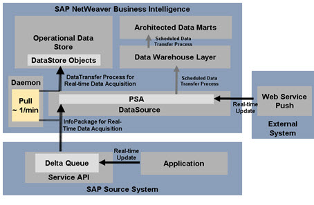
G.                Data Acquisition.

Data retrieval is one of the data warehousing processes in BI. BI provides mechanisms for retrieving data (master data, transaction data, and metadata) from various sources. The following sections describe the sources available for the data transfer to BI and how the sources are connected to the BI system as source systems. They also describe how the data can be transferred from the sources.

The extraction and transfer of data generally occurs upon request of BI (pull). The sections about the scheduler, process chain and monitor describe how such a data request is defined and how the load process can be monitored in the BI system.

The graphic shows the sources and transfer mechanisms described below:

All systems that provide BI with data are described as source systems. These can be:

• SAP Source System.

The SAP BW service API (Application Programming Interface) is based exclusively on SAP technology and is used at various points within the SAP BW architecture to transfer data and metadata from SAP source systems.

• Flat files for which metadata maintained manually and transferred to BW is using a file interface. Flat files source systems used for uploading flat files in ASCII, CSV (comma separated variables), or binary format.
• Database management systems into which data is loaded from a database supported by SAP using DB Connect, without using an external extraction program.
• Relational or multidimensional sources that are connected to BI using UD Connect.
• Web Services that transfer data to BI by means of a push.
• Non – SAP systems for which data and metadata is transferred using staging BAPIs (no staging BAPI available for new datasources).

H.                Migration DataSources.

You can migrate a 3.x DataSource that transfers data into BI from an SAP source system or a file or uses DB Connect to transfer data into a DataSource.  3.x XML DataSources and 3.x DataSources that use UD Connect to transfer data cannot be migrated directly. However, you can use the 3.x versions as a copy template for a Web service or UD Connect DataSource (note: You cannot migrate hierarchy DataSources, DataSources that use the IDoc transfer method, export DataSources (namespace 8* or /*/8*) or DataSources from BAPI source systems).

Below explain the procedure to migrating 3.x DataSources:

• In the Data Warehousing Workbench, choose Migrate in the context menu of the 3.x DataSource.

• If you want to restore the 3.x DataSource at a later time, choose With Export on the next screen.

I.                   Transformation.

The transformation process allows you to consolidate, cleanse, and integrate data. You can semantically synchronize data from heterogeneous sources. When you load data from one BI object into a further BI object, the data is passed through a transformation. A transformation converts the fields of the source into the format of the target. You create a transformation between a source and a target. The BI objects DataSource, InfoSource, DataStore object, InfoCube, InfoObject and InfoSet serve as source objects. The BI objects InfoSource, InfoObject, DataStore object and InfoCube serve as target objects. The following graphic illustrates how the transformation is integrated in the dataflow:

A transformation consists of at least one transformation rule. Various rule types, transformation types, routine types, and transformation group are available.

1. 1.         Rule Types.

The rule type determines whether and how a characteristic/key figure or a data field/key field is updated into the target. The following options are available:

• Direct Assignment.

The field is filled directly from the chosen source InfoObject. If the system does not propose a source InfoObject, you can assign a source InfoObject of the same type (amount, number, integer, quantity, float, time) or create a routine.

• Constant.

The field is not filled by the InfoObject but is filled directly with the value specified.

• Formula.

The InfoObject is updated with a value determined using a formula.

• Reading Master Data.

The InfoObject is updated by reading the master data table of a characteristic that is included in the source with a key and a value and contains the corresponding InfoObject as an attribute. The attributes and their values are read from the key, these are then returned. If the attribute is time dependent, you also have to define when it should be read: at the current date (sy-date), at the beginning or end of a period (defined by a time characteristic in the InfoSource), or at a constant date that you enter directly. Sy-date is used as the default.

• Routine.

The field is filled by the transformation routine you have written. The system offers you a selection option that lets you decide whether the routine is valid for all of the attributes belonging to this characteristic, or only for the attributes displayed.

• Initial.

The field is not filled. It remains empty.

• No Transformation.

The key figures are not written to the InfoProvider.

1. 2.         Transformation Types.

The transformation type determines how data is written into the fields of the target. You use the aggregation type to control how a key figure or data field is updated to the InfoProvider.

• For InfoCube.

Depending on the aggregation type you specified in key figure maintenance for this key figure, you have the options Summation, or Maximum or Minimum. If you choose one of these options, new values are updated to the InfoCube.

• For InfoObject.

Only the Overwrite option is available. With this option, new values are updated to the InfoObject.

• For DataStore Object.

Depending on the type of data and the DataSource, you have the options Summation, Minimum, Maximum or Overwrite. When you choose one of these options, new values are updated to the DataStore object.

1. 3.         Routine.

Routines used to define complex transformation rules. Routines are local ABAP classes that consist of a predefined definition area and an implementation area. The TYPES for the inbound and outbound parameters and the signature of the method are determined in the definition area. The actual routine is created in the implementation area. In the method, ABAP object statements are available. Upon generation, this method is embedded in the local class of the transformation program. The following graphic shows the position of these routines in the data flow:

Transformations include different types of routine:

• Start Routines.

The start routine is run for each data package at the start of the transformation. The start routine does not have a return value. It is used to perform preliminary calculations, preparation of data before transformation and store these in a global data structure or in a table. You can access this structure or table from other routines. You can modify or delete data.

• End Routines.

An end routine is a routine with a table in the target structure format as an input parameter and an output parameter. An end routine used to execute the post-processing of data after transformation on a package-by-package basis. For example, you can delete records that are not to be updated, or perform data checks.

• Expert Routines.

This type of routine is only intended for use in special cases. You can use the expert routine if there are not sufficient functions to perform a transformation. You can use the expert routine as an interim solution until the necessary functions are available in the standard routine. You can use this to program the transformation yourself without using the available rule types. You must implement the message transfer to the monitor yourself. If you have already created transformation rules, the system deletes them once you have created an expert routine.

1. 4.         Transformation Groups.

Transformation Groups replaces the former concept of key figure-specific updates for the characteristic. In 3.x you could define characteristic updates per key figure. In most cases this was the same for all key figures. To define one key figure different to the others you would in B.I 7.0 use the concept of transformation groups. A standard group exists. If you change this all referencing groups could be changed as well.

J.                  Transformation – Info Source.

The InfoSource is not mandatory anymore. You use InfoSources if you want to run two (or more) sequential transformations in the data flow, without storing the data again. f you do not have transformations that run sequentially, you can model the data flow without InfoSources. In this case, the data is written straight to the target from the source using a transformation.

However, it may be necessary to use one or more InfoSources for semantic or complexity reasons. For example, you need one transformation to ensure the format and the assignment to InfoObjects and an additional transformation to run the actual business rules. If this involves complex inter-dependent rules, it may be useful to have more than one InfoSource.

This section outlines three scenarios for the use of InfoSources. The decision whether or not to use an InfoSource depends on how the work required maintaining any potential changes required in the scenario can be minimized.

1. 1.      Data Flow without an InfoSource.

The DataSource is connected directly to the target by means of a transformation. Since there is only one transformation to be passed through, the performance is better.

1. 2.      Data Flow with One InfoSource.

The DataSource is connected to the target by means of a InfoSource. There is one transformation between the DataSource and the InfoSource, and one transformation between the InfoSource and the target.

It is advisable to use an InfoSource when multiple different DataSources, to which the same business rules are to apply, are to be connected to a target. You can align the format of the data in the transformation between the DataSource and InfoSource. The required business rules are executed in the subsequent transformation between the InfoSource and the target. If required, you can make any necessary changes to these rules centrally in this one transformation.

1. 3.      Data Flow with Two InfoSource.

We recommend you use this type of data flow if your data flow not only contains two different sources, but the data is to be written to multiple identical (or almost identical) targets. The necessary business rules are executed in the central transformation, such that any changes to the sources or the targets only require you to adjust the one transformation accordingly.

 

 

K.                Data Transfer Process (DTP).

Data Transfer Process (DTP) is object that determines how data is transferred between two persistent objects. You use the data transfer process (DTP) to transfer data within BI from a persistent object to another object in accordance with certain transformations and filters. In this respect, it replaces the data mart interface and the InfoPackage. As of SAP NetWeaver 2004s, the InfoPackage only loads data to the entry layer of BI (PSA).

Benefits of new Data Transfer Process (DTP):

• Loading data from one layer to others except InfoSources.
• Separation of delta mechanism for different data targets.
• Enhanced filtering in dataflow.
• Improved transparency of staging processes across data warehouse layers (PSA, DWH layer, ODS layer, Architected Data Marts).
• Improved performance: optimized parallelization.
• Enhanced error handling for DataStore Object (Error stack).
• Enables real-time data acquisition.

• Filter In Data Transfer Process (DTP).

With the extraction mode, you can decide whether the Data Transfer Process loads the data in ‘Full’ or ‘Delta’ mode. For the delta loading, you need to define two Data Transfer Processes (one ‘Full’ and one ‘Delta’ DTP) to load the data from source to target.

With the filter function it is possible to load a set of data to the data target instead of the complete volume of data. Different data selections can be made via different Data Transfer Process for the same or for different data targets. You can define the package size, whether the currency conversion should be switched on or whether it is possible to load the data from the change log of the DataStore Object. Regarding the update mode and execution mode we first need to look into error handling features of DTP.

This slide illustrates how error handling works with the DTP. You have the option to choose whether you want to switch on the error handling feature or not. If you choose option 2 or 3 it will works as follow:

• Data is loaded via InfoPackage from Source System to PSA table. There is no error handling available for InfoPackage. In case of invalid records data needs to be reloaded from the Source System.
• You can load the data from OPSA to Data Target via DTP. As you have switched on the error handling features, the invalid records will be updated into the error stack. The correct records will be updated into the data target. After you have corrected the records in the error stack, you can load these corrected data records to the data target via “Error DTP’. This is special DTP which is responsible or loading data from the error stack to the data target.